Transformation from camera coordinate frame to body coordinate frame

In here I describe how to transform the coordinates of a given point in camera coordinate frame into body coordinate frame. I am still confused with the concept of vectors, matrices, coordinate systems and transformations. I feel I am lacking some intuition. I also realise I may not need a transformation at all given that I will not use the coordinates of the joints as features but instead use the differences (length and angles) between them — that way, transformation is irrelevant. Nevertheless, here’s what I will take note of. A few helpful references for matrix transformation is given under the background knowledge section.

Summary

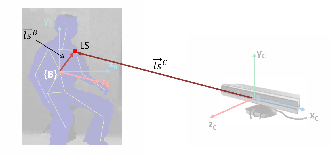
The idea is to transform the coordinate frame from camera {C} to the torso joint of the first frame {B}.

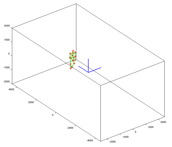
First obtain the following joint coordinates from the first frame of an activity instance captured from Kinect (i.e. in {C} ). Note I have chosen to define the body coordinate frame at the torso joint in first frame.

torso joint

(1) $\begin{equation*} \vec { t }(1) = \begin{bmatrix} { t }_{ x }(1) \\ { t }_{ y }(1) \\ { t }_{ z }(1) \end{bmatrix} \end{equation*}$

left shoulder joint

(2) $\begin{equation*} \vec { ls }(1) = \begin{bmatrix} { ls }_{ x }(1) \\ { ls }_{ y }(1) \\ { ls }_{ z }(1) \end{bmatrix} \end{equation*}$

right shoulder joint

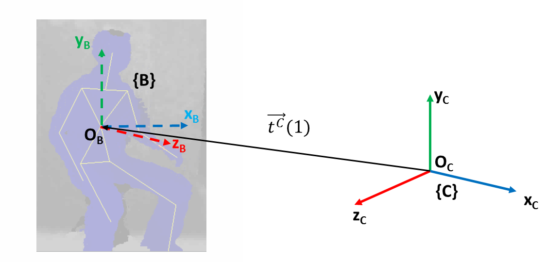
(3) $\begin{equation*} \vec { rs }(1) = \begin{bmatrix} { rs }_{ x }(1) \\ { rs }_{ y }(1) \\ { rs }_{ z }(1) \end{bmatrix} \end{equation*}$

Second, form the transformation matrix (in homogeneous form, i.e. 4×4) to translate the origin from {B} to the origin of {C}. Here’s we use the position of the torso joint. Note the translation is the reverse of the torso joint vector. This translation effectively moves the position of {B} to {C}. Imagine moving the person in the image above to the center of the Kinect.

(4) $\begin{equation*} { T(trans) }_{ C }^{ B }= \begin{bmatrix} 1 & 0 & 0 & -{ t }_{ x }(1) \\ 0 & 1 & 0 & -{ t }_{ y }(1) \\ 0 & 0 & 1 & -{ t }_{ z }(1) \\ 0 & 0 & 0 & 1 \end{bmatrix} \end{equation*}$

Third, obtain the unit vectors of the x-axes of two reference frames from the vectors of the left and right shoulder joints. For {B}, we assume the x-axis is along the shoulder pointing to the left of the person. Unit vector is computed from the difference between the two shoulder vectors normalized to unit length. For {C}, it is simply a unit length vector pointing in x-axis of {C}.

(5) $\begin{equation*} \hat { { x }_{ B' } } =\frac { 1 }{ \left\| { \left( \vec { ls }(1) -\vec { rs }(1) \right) }_{ y=0 } \right\| } { \left( \vec { ls }(1) -\vec { rs }(1) \right) }_{ y=0 }\quad and\quad \hat { { x }_{ C } } = \begin{bmatrix} 1 \\ 0 \\ 0 \end{bmatrix} \end{equation*}$

Forth, compute the rotation angle $\theta$ as the angle between the two unit x-axes vectors. We use the inverse cosine of the dot product of the two unit vectors to determine the angle between them, and treated the sign such that it will rotate ${x}_{c}$ into the orientation of ${x}_{b}$ .

(6) $\begin{equation*} \theta =sign\left( { \left( \hat { { x }_{ B' } } \times \hat { { x }_{ C } } \right) }_{ y } \right) { cos }^{ -1 }\left( \hat { { x }_{ B' } } \cdot \hat { { x }_{ C } } \right) \end{equation*}$

Fifth, form the homogeneous transformation matrix for rotation that would rotate ${x}_{c}$ into the orientation of ${x}_{b}$ .

(7) $\begin{equation*} { T(rot) }_{ C }^{ B }= \begin{bmatrix} cos\theta & 0 & sin\theta & 0 \\ 0 & 1 & 0 & 0 \\ -sin\theta & 0 & cos\theta & 0 \\ 0 & 0 & 0 & 1 \end{bmatrix} \end{equation*}$

Sixth, compose the homogeneous transformation matrix ${ T }_{ C }^{ B }$ ,

(8) $\begin{equation*} { T }_{ C }^{ B }={ T }(rot)_{ C }^{ B }{ *T(trans) }_{ C }^{ B } \end{equation*}$

Finally, given a point P whose coordinates in {C} is given by

(9) $\begin{equation*} \vec { { p }^{ C } } = \begin{bmatrix} { p }_{ x }^{ C } \\ { p }_{ y }^{ C } \\ { p }_{ z }^{ C } \end{bmatrix} \end{equation*}$

Pad the vector and compute its coordinates in {B} ,

(10) $\begin{equation*} \begin{bmatrix} \vec { { p }^{ B } } \\ 1 \end{bmatrix} = \begin{bmatrix} { p }_{ x }^{ B } \\ { p }_{ y }^{ B } \\ { p }_{ z }^{ B } \\ 1 \end{bmatrix} ={ T }_{ C }^{ B }[ \begin{bmatrix} \vec { { p }^{ C } } \\ 1 \end{bmatrix} \end{equation*}$

Details

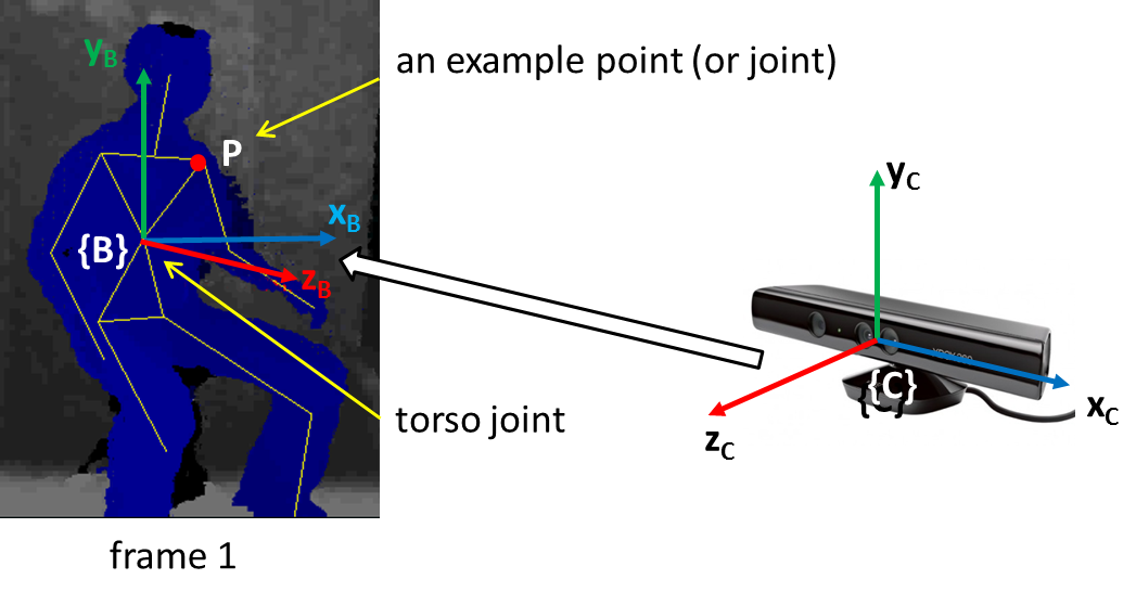
First, I note the coordinate frame of Kinect is right handed . (NOTE: I can’t confirm this info. Microsoft document says it is right handed, however my system with SimpleOpenni is left handed, i.e. x value increases toward right of sensor. Anyway, the following discussion remains valid. Only that if it was left handed, then the resulting local coordinate system will also be left handed. I also note OpenNI called our left as right and vice versa, i.e. our right hand is the left hand in OpenNI.) The origin is right at the center of its face. z-axis increases when moving away from the face; y-axis increases upward; x-axis increases to its left (viewer’s right). Lets call this camera coordinate frame {C} .

I want to define a body coordinate frame, lets call it {B} , on the detected human skeleton from Kinect API. I decided to place {B} at the torso joint of the first frame of an activity instance. Alternatively, I could have place {B} at the torso joint of each frame. By doing so, I would need to compute the transformation matrix in each frame and the location of the person would appear stationary; I would require additional feature to capture the movement with respect to the world. Note that an activity instance comprises series of frames of posture.

To simplify the transformation, I maintain the y-axis in {B} parallel to y-axis in {C} , i.e. pointing upward. Also, the x-z plane in {B} is parallel to that in {C} . In this way, the required transformation comprises (only) of a rotation around y-axis in {C} to align {B} such that its z-axis is pointing to the front of the person and a translation from origin of {C} , i.e. <0,0,0> to the torso joint position in the first frame.

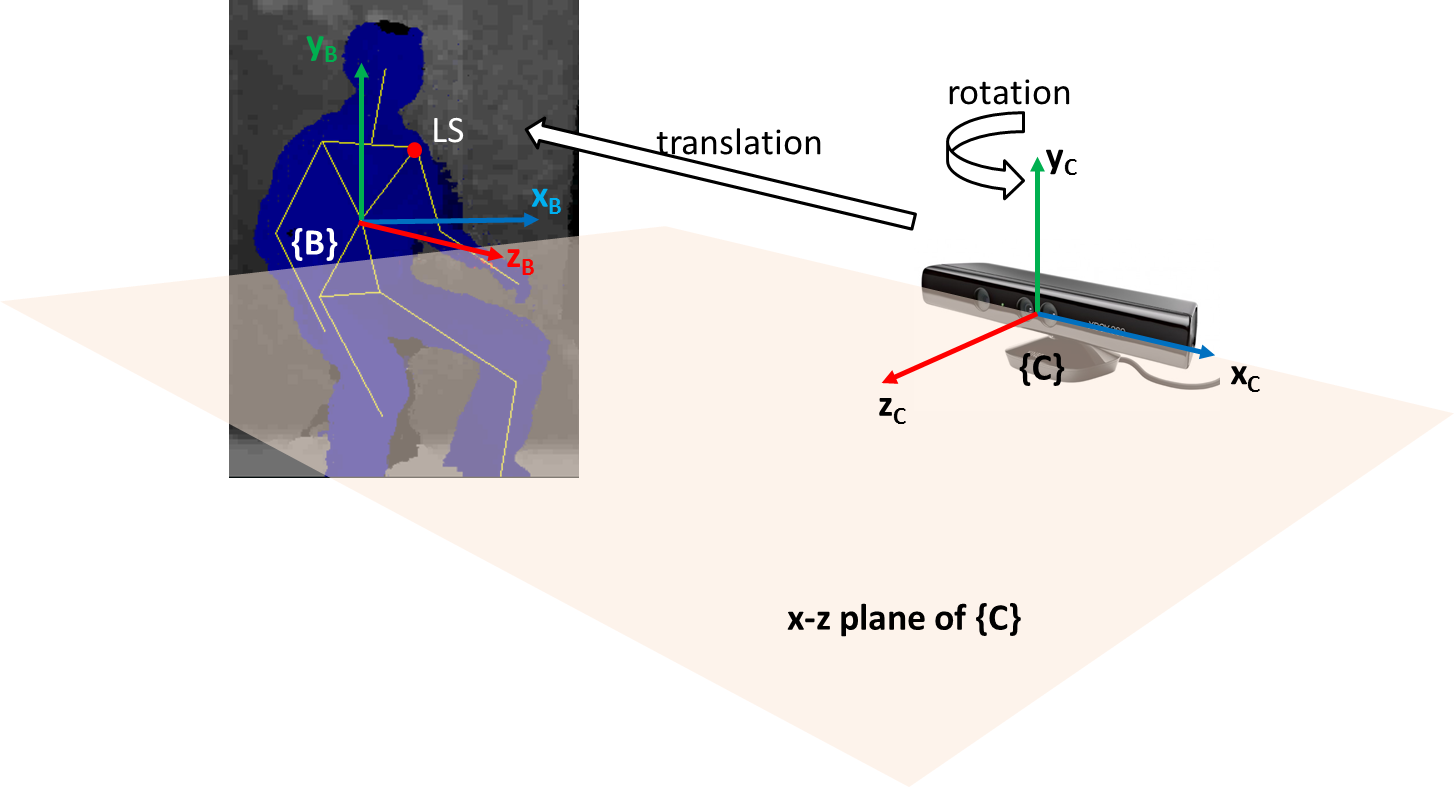
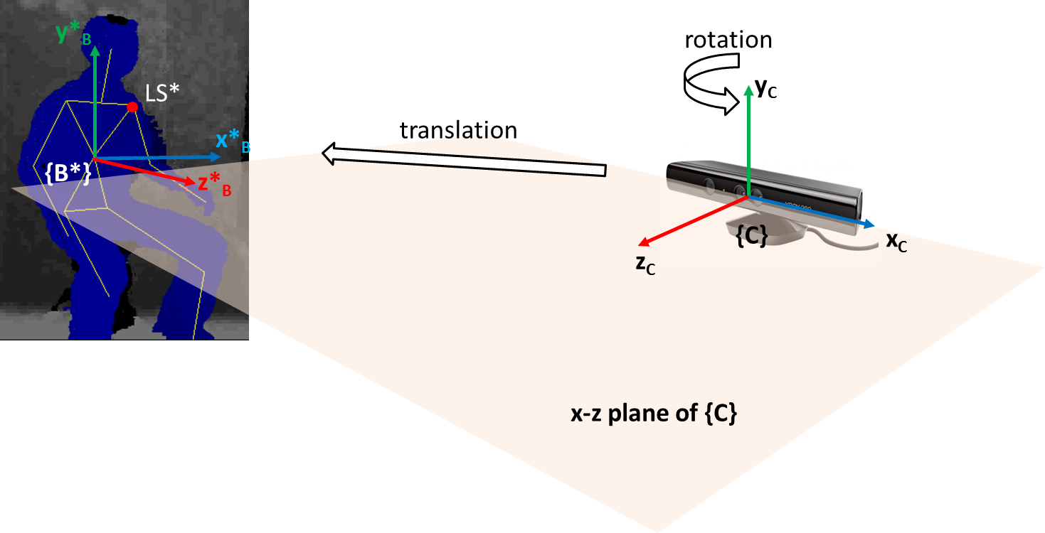
Note in the above two figures, the relative positions between the person and the camera are different, i.e. the camera is looking from different view points. However, the person is in same posture. Before any transformation (in {C} ), the coordinates of any joint (e.g. the left shoulder LS ) will be different in the two scenarios. Whereas if the coordinate frame is transformed to the body, {B} , the coordinates of $\vec { ls }$ and $\vec { ls* }$ (these are the vectors from the origin of the reference frame to the point LS and LS* respectively), for example, are the same. In this way, the coordinates are view-invariant and we can better recognise similar postures. In equations below, superscript is used to indicate the reference coordinate frame.

(11) $\begin{equation*} \vec{ { ls } ^{ C } } \neq { \vec{ { ls* }^{ C } }\end{equation*}$

(12) $\begin{equation*} \vec {{ ls } ^{ B }}= \vec {{ ls* } ^{ B* }} \end{equation*}$

To transform the coordinates of a point in {C} , $\vec {{ p } ^{ C }}$ , to coordinates in {B} , $\vec {{ p } ^{ B }}$ , we need to determine the homogeneous transformation matrix , ${ T }_{ C }^{ B }$ such that:

(13) $\begin{equation*} \vec {{ p } ^{ B }}={ T }_{ C }^{ B } \vec{ { p } ^{ C } }\end{equation*}$

where,

(14) $\begin{equation*} { T }_{ C }^{ B }={ F }_{ B }^{ C } \end{equation*}$

For example $\vec{ { ls } ^{ B }}={ T }_{ C }^{ B }\vec{ { ls } ^{ C }}$ .

${ F }_{ B }^{ C }$ is the required transformation to move {B} such that it aligns with {C} . Note when labeling axes and components, I have used superscripts, e.g. ${ x }_{ C }$ is the x-axis of {C} ; ${ d }_{ x }$ is the x-component of vector $\vec{ d }$ .

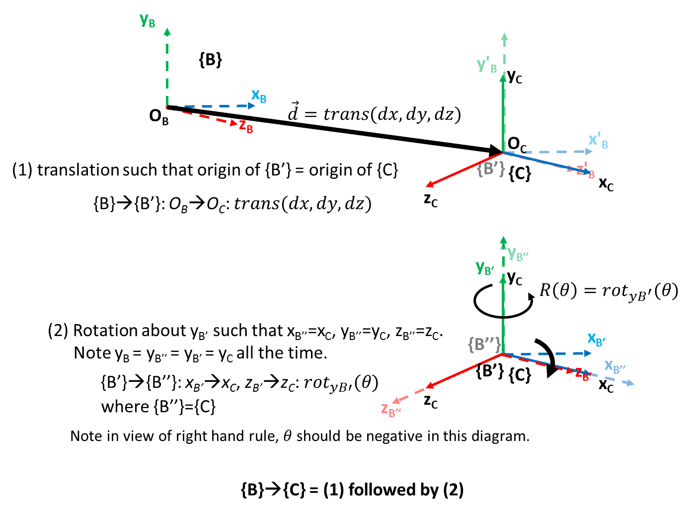
Note that, the sequence of operations can be reversed, i.e. rotation first then translation. In both ways, we should obtain the same ${ F }_{ B }^{ C }$ , however the order of composing ${ F }_{ B }^{ C }$ must be second operation multiply by first (2)*(1). Further, if we do the rotation first, we would be rotating around the y-axis of {C} since we are using the coordinates from {C}. This would not give the desired effect to align the body’s front to z-axis. I will do translation followed by rotation.

The translation, ${ \vec { d } }$ is simply the reverse of the torso joint vector ${ \vec { { t }^{ C } }(1) }$ in first frame. Note (1) is used to indicate frame 1 .

(15) $\begin{equation*} { \vec { d } =-\vec { { t }^{ C } }(1) =-\left< { t }_{ x }^{ C }(1),{ t }_{ y }^{ C }(1),{ t }_{ z }^{ C }(1) \right> =-\begin{bmatrix} { t }_{ x }^{ C }(1) \\ { t }_{ y }^{ C }(1) \\ { t }_{ z }^{ C }(1) \end{bmatrix} } \end{equation*}$

The translation can be expressed in homogeneous form,

(16) $\begin{equation*} { T(trans) }_{ C }^{ B }= \begin{bmatrix} 1 & 0 & 0 & -{ t }_{ x }(1) \\ 0 & 1 & 0 & -{ t }_{ y }(1) \\ 0 & 0 & 1 & -{ t }_{ z }(1) \\ 0 & 0 & 0 & 1 \end{bmatrix} \end{equation*}$

After the translation, the origin of {B} and {C} are aligned (y-axes are aligned). However, a rotation is required to align the other two axes. The rotation matrix around y-axis to move the x and z-axes (considered as vectors in this movement) in { B' } to align with corresponding axes in { C } (i.e. such that { B'' }={ C } ) is given by:

(17) $\begin{equation*} R(\theta )= \begin{bmatrix} cos\theta & 0 & sin\theta \\ 0 & 1 & 0 \\ -sin\theta & 0 & cos\theta \end{bmatrix} \end{equation*}$

The following diagram shows the necessary vectors to determine $\theta$ . I basically use the vector connecting left and right shoulder joints to determine the direction of x-axis in { B' } ( $\hat { { x }_{ B' } }$ ) and then use dot product to computer the angle $\theta$ between it and the original x-axis in { C } ( $\hat { { x }_{ C } }$ ).

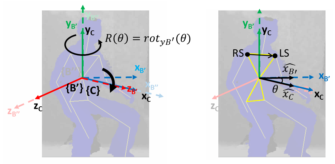
$\hat { { x }_{ B' } }$ and $\hat { { x }_{ C } }$ are unit vectors in the direction of ${ x }_{ B' }$ and ${ x }_{ C }$ axes respectively. The value of $\theta$ can be determined using dot product and the criteria that $\hat { { x }_{ B' } }$ stays on (parallel to) the x-z plane. Since it is expected that the data for computation will be with reference to {C} (fromKinect), all values are taken with reference to {C} .

(18) $\begin{equation*} \hat { { x }_{ B' } } \cdot \hat { { x }_{C } } =\left| \hat { { x }_{ B' } } \right| \left| \hat { { x }_{ C } } \right| cos\theta \end{equation*}$

Since, $\left| \hat { { x }_{ B' } } \right|$ and $\left| \hat { { x }_{ C } } \right|$ are unit length, and $\hat { { x }_{ C } } = \begin{bmatrix} 1 \\ 0 \\ 0 \end{bmatrix}$ with reference to {C} , we have

(19) $\begin{equation*} \begin{align*} cos\theta & = & \hat { { x }_{ B' } } \cdot \hat { { x }_{ C } } \\ & = & \hat { { x }_{ B' } } \cdot \begin{bmatrix} 1 \\ 0 \\ 0 \end{bmatrix} \end{align*} \end{equation*}$

Note the use of cosine makes the sign of $\theta$ irrelevant. However, the sign will be needed eventually when computing the sines. To determine $\hat { { x }_{ B' } }$ , we note $\hat { { x }_{ B' } }$ is parallel to $\vec { ls } -\vec { rs }$ ( $\vec{ls}$ and $\vec{rs}$ are vectors from origin to LS and RS respectively). Further, when parallel to x-z plane, the y-component is made zero.

(20) $\begin{equation*} \hat { { x }_{ B' } } =k{ \left( \vec { ls }(1) -\vec { rs }(1) \right) }_{ y=0 }\\ =k \begin{bmatrix} { ls }_{ x }(1)-{ rs }_{ x }(1) \\ 0 \\ { ls }_{ z }(1)-{ rs }_{ z }(1) \end{bmatrix} \end{equation*}$

To find k , we note $\hat { { x }_{ B' } }$ is unit vector, i.e. has unit magnitude.

(21) $\begin{equation*} \begin{align*} \left\| k{ \left( \vec { ls }(1) -\vec { rs }(1) \right) }_{ y=0 } \right\| & = & 1 \\ k & = & \frac { 1 }{ \left\| { \left( \vec { ls }(1) -\vec { rs }(1) \right) }_{ y=0 } \right\| } \end{align*} \end{equation*}$

From (19), (20) and (21), we have

(22) $\begin{equation*} \hat { { x }_{ B' } } =\frac { 1 }{ \left\| { \left( \vec { ls }(1) -\vec { rs }(1) \right) }_{ y=0 } \right\| } { \left( \vec { ls }(1) -\vec { rs }(1) \right) }_{ y=0 }\quad and\quad \hat { { x }_{ C } } = \begin{bmatrix} 1 \\ 0 \\ 0 \end{bmatrix} \end{equation*}$

(23) $\begin{equation*} \theta ={ cos }^{ -1 }\left( \hat { { x }_{ B' } } \cdot \hat { { x }_{ C } } \right) \end{equation*}$

Note the two vectors in (23) are operated by dot product. In (23), I do not have the sign of $\theta$ . To determine, the sign of $\theta$ , I use the cross product of $\hat { { x }_{ B' } }$ and $\hat { { x }_{ C } }$ . Note right handed rule being applied to determine positive direction, as well as the resultant vector of cross product.

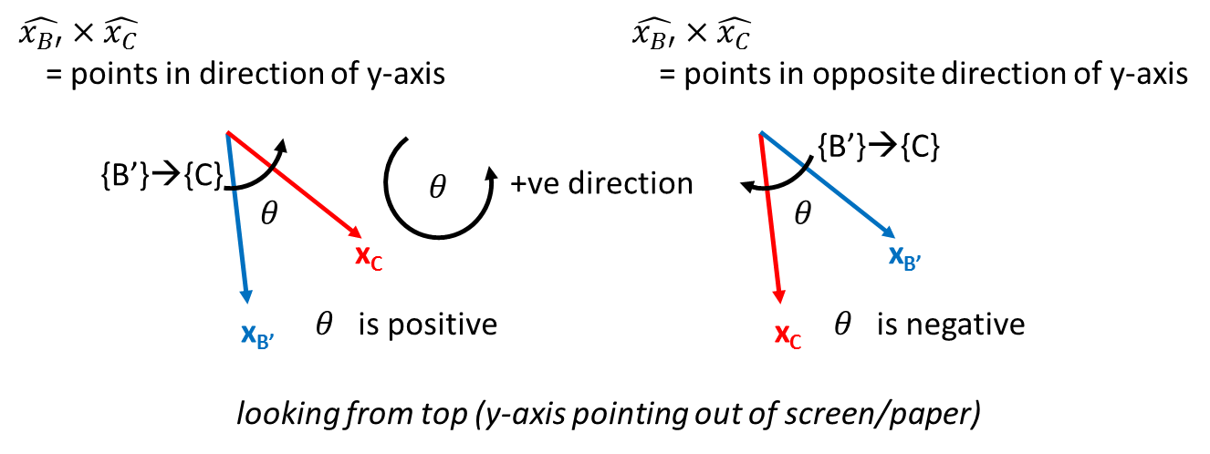
From the above diagram, if the result of the cross product is in the direction of y-axis, $\theta$ is positive, otherwise $\theta$ is negative. Therefore, $\theta$ has the sign of the y-component of $\hat { { x }_{ B' } } \times \hat { { x }_{ C } }$ . Note also the x and z components of the cross-product are expected to be zero (since it is along y-axis).

(24) $\begin{equation*} \theta =sign\left( { \left( \hat { { x }_{ B' } } \times \hat { { x }_{ C } } \right) }_{ y } \right) { cos }^{ -1 }\left( \hat { { x }_{ B' } } \cdot \hat { { x }_{ C } } \right) \end{equation*}$

With (15) and (17), we can transform the the coordinates of a point in {C} , $\vec {{ p } ^{ C }}$ , to coordinates in {B} , $\vec {{ p } ^{ B }}$ ,

(25) $\begin{equation*} \vec {{ p } ^{ B }}={ T }_{ C }^{ B } \vec{ { p } ^{ C } }\end{equation*}$

where,

(26) $\begin{equation*} { T }_{ C }^{ B }={ T }(rot)_{ C }^{ B }{ *T(trans) }_{ C }^{ B } \end{equation*}$

and $\theta$ is given in (24) and, ${ t }_{ x }(1)$ , ${ t }_{ y }(1)$ and ${ t }_{ z }(1)$ are the coordinates of the torso joint in first frame. To use the 4×4 transformation matrix, the coordinates of a vector in {C} must be padded:

(27) $\begin{equation*} \vec { { p }^{ C } } = \begin{bmatrix} { p }_{ x } \\ { p }_{ y } \\ { p }_{ z } \\ 1 \end{bmatrix} \end{equation*}$

The resultant vector will be 4×1 and the padded 4th element can be removed to obtain a 3×1 vector (just the x, y and z components). Note all coordinates are reference to {C}.

Octave implementation

Here’s the Octave implementation for the transformation, including codes to transform all examples (instances) in a given file.

Background knowledge

I found the note on homogeneous transform by Jennifer Kay from Rowan University being most readable for novice like myself. Jennifer uses good number of illustrations and simple examples to explain the concepts of coordinate transformation and its application in forward kinematic in robotic arm. There are a number of things I found difficult to grasp when reading her note, here are a few:

The arrangement of the axes are different from my familiar Kinect coordinate system, i.e. y-axis is pointing upward; however, this is normal as different systems adopt different axes arrangement.
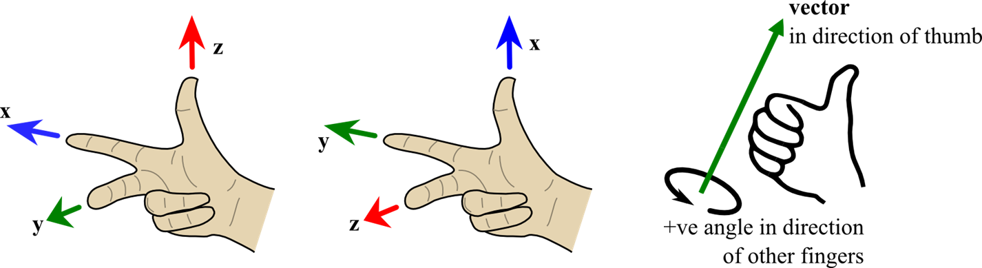
The explanation of right hand rule seems a little complicated; it is sufficient to use the following diagrams to explain right hand rule to determine the relative position of the axes as well as the positive rotation direction.
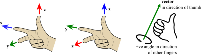
Right hand rule: note there is no consistency in assignment of axes to fingers, however it is the order that matters.
The elements used in the homogeneous transformation matrix are not given explanation, i.e. “this are the formulas, and trust it”. Likewise, the note started by using a four coordinates to represent a point, which was difficult to appreciate the extra “weight” component. It helps to ask ourselves to not be curious, at this point, about how those cosines, sines and their arrangement in a 4×4 matrix come from. Just take it for now as we can then clearly see that they work. In that sense, we can quickly use it in our application. We can then probe further to understand homogeneous transformation .

[gview file=”http://elvis.rowan.edu/~kay/papers/kinematics.pdf”]

Jennifer’s note is based on the tutorial ” Essential Kinematics for Autonomous Vehicles ” (this is later version) by Alonzo Kelly from CMU, which I found Jennifer has done an excellent job to explain clearly. To probe further on how homogeneous transformation matrix is derived, I found the note on Kown3D quite easy to digest.

Kown3D also explains the difference between rotating axis (coordinate frame rotation) and rotating a vector (no change to coordinate frame) , which is an important concept to grasp to under the concept of transformation.

Still, I haven’t fully understand everything explained. One the problem was my lack of understanding or intuition of dot production and vectors. The videos on Khan Academy explain some of these concepts well.

Here’s explanation of cross product.

Files

TODO**: Instructions on how to use.

Octave file transformAllToFirstFrameF.m (function)
Files to draw the skeleton before and after transformation (takes the Xsamp or XsampT files): drawSkeleton.m and drawSkeletonForOneExample.m (called by drawSkeleton.m)